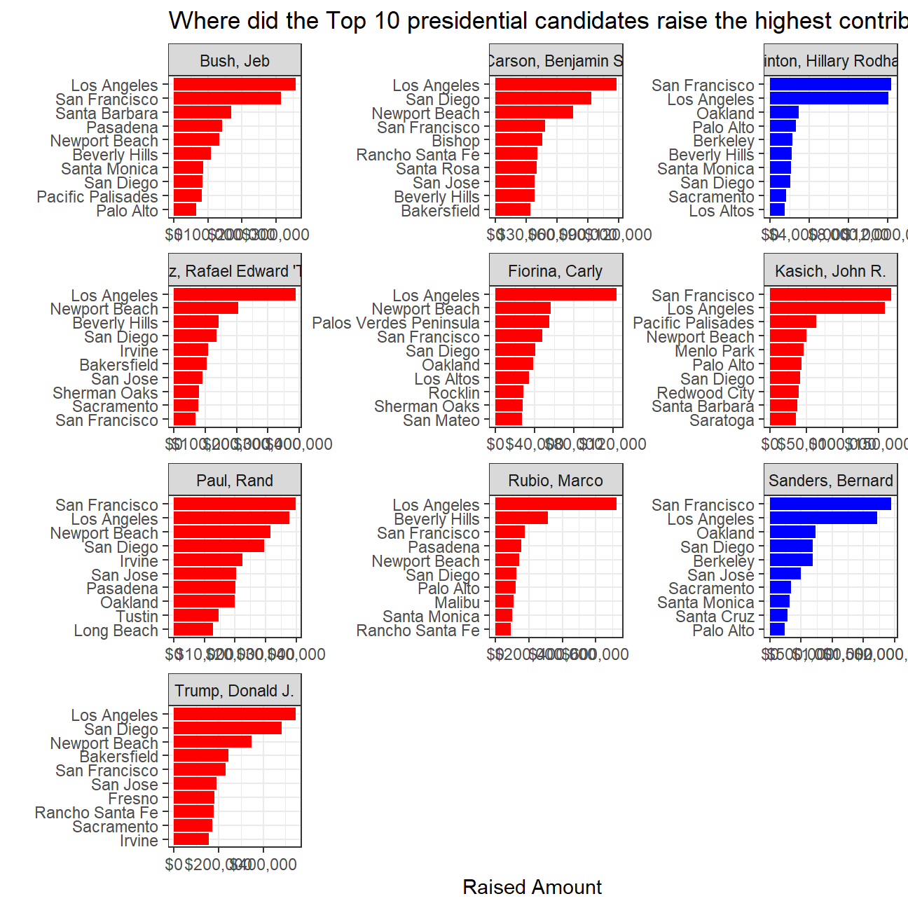
Cities with the highest amounts in political contributions in California during the 2016 US Presidential election
As discussed in class, I would like you to reproduce the plot that shows the top ten cities in highest amounts raised in political contributions in California during the 2016 US Presidential election.

CA_contributors_2016 <- vroom::vroom(here::here("data","CA_contributors_2016.csv"))
Zip_codes <- vroom::vroom(here::here("data","zip_code_database.csv"))

Zip_codes_clean <- filter(Zip_codes, state == "CA")

Cali_contributors <- CA_contributors_2016 %>%
  filter(cand_nm %in% c("Clinton, Hillary Rodham","Trump, Donald J."))

joint_zip <- merge(Cali_contributors, Zip_codes_clean, "zip")

new_data <- joint_zip %>%
  group_by(cand_nm) %>%
  count(primary_city, wt = contb_receipt_amt, sort = TRUE)

new_data %>%
  group_by(cand_nm) %>%
  top_n(10) %>%
  ungroup %>%
  mutate(cand_nm = factor(cand_nm),
    primary_city = reorder_within(primary_city, n, cand_nm)) %>%
  ggplot(aes(x = primary_city, y = n, fill = cand_nm)) +
  geom_col(show.legend = FALSE) +

  scale_fill_manual(values = c("Clinton, Hillary Rodham" = "blue","Trump, Donald J." = "red")) +
  facet_wrap(~cand_nm, scales = 'free') +
  scale_x_reordered() +
  scale_y_continuous(labels = label_dollar()) +
  theme_bw() +
  labs(y = "Raised Amount",
       x = "",
       title = "Where did the candidates raise most of their money?") +
coord_flip() 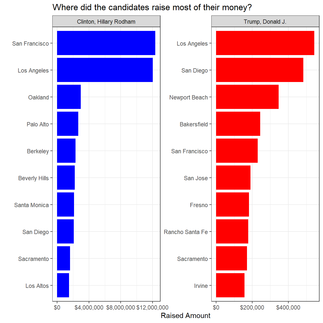
CA_contributors_top10 <- CA_contributors_2016 %>%
  group_by(cand_nm) %>%
  summarise(total_contr = sum(contb_receipt_amt)) %>%
  arrange(desc(total_contr)) %>%
  head(10)
top10_contributors <- CA_contributors_top10$cand_nm

Cali_top_10 <- CA_contributors_2016 %>%
  filter(cand_nm %in% top10_contributors)

merged_top_10 <- merge(Cali_top_10,Zip_codes_clean,"zip")


total_data <- merged_top_10 %>%
  group_by(cand_nm) %>%
  count(primary_city, wt = contb_receipt_amt, sort = TRUE)

candm_shade <- c("Bush, Jeb"  = "red",
                 "Carson, Benjamin S." ="red",
                 "Clinton, Hillary Rodham" = "blue",
                 "Cruz, Rafael Edward 'Ted'" ="red",
                 "Fiorina, Carly" ="red",
                 "Kasich, John R." ="red",
                 "Paul, Rand" ="red",
                 "Rubio, Marco" ="red",
                 "Sanders, Bernard" = "blue",
                 "Trump, Donald J." = "red")

total_data %>%
  group_by(cand_nm) %>%
  top_n(10) %>%
  ungroup %>%
  mutate(cand_nm = factor(cand_nm),
    primary_city = reorder_within(primary_city, n, cand_nm)) %>%
  ggplot(aes(x = primary_city, y = n, fill = cand_nm)) +
  geom_col(show.legend = FALSE) +
  scale_fill_manual(values = candm_shade) +
  facet_wrap(~cand_nm, scales = "free",nrow = 4, ncol = 3) +
  scale_x_reordered() +
  scale_y_continuous(labels = label_dollar()) +
  theme_bw() +
  labs(y = "Raised Amount",
       x = "",
       title = "Where did the Top 10 presidential candidates raise the highest contributions?") +
  coord_flip()